Month: June 2021

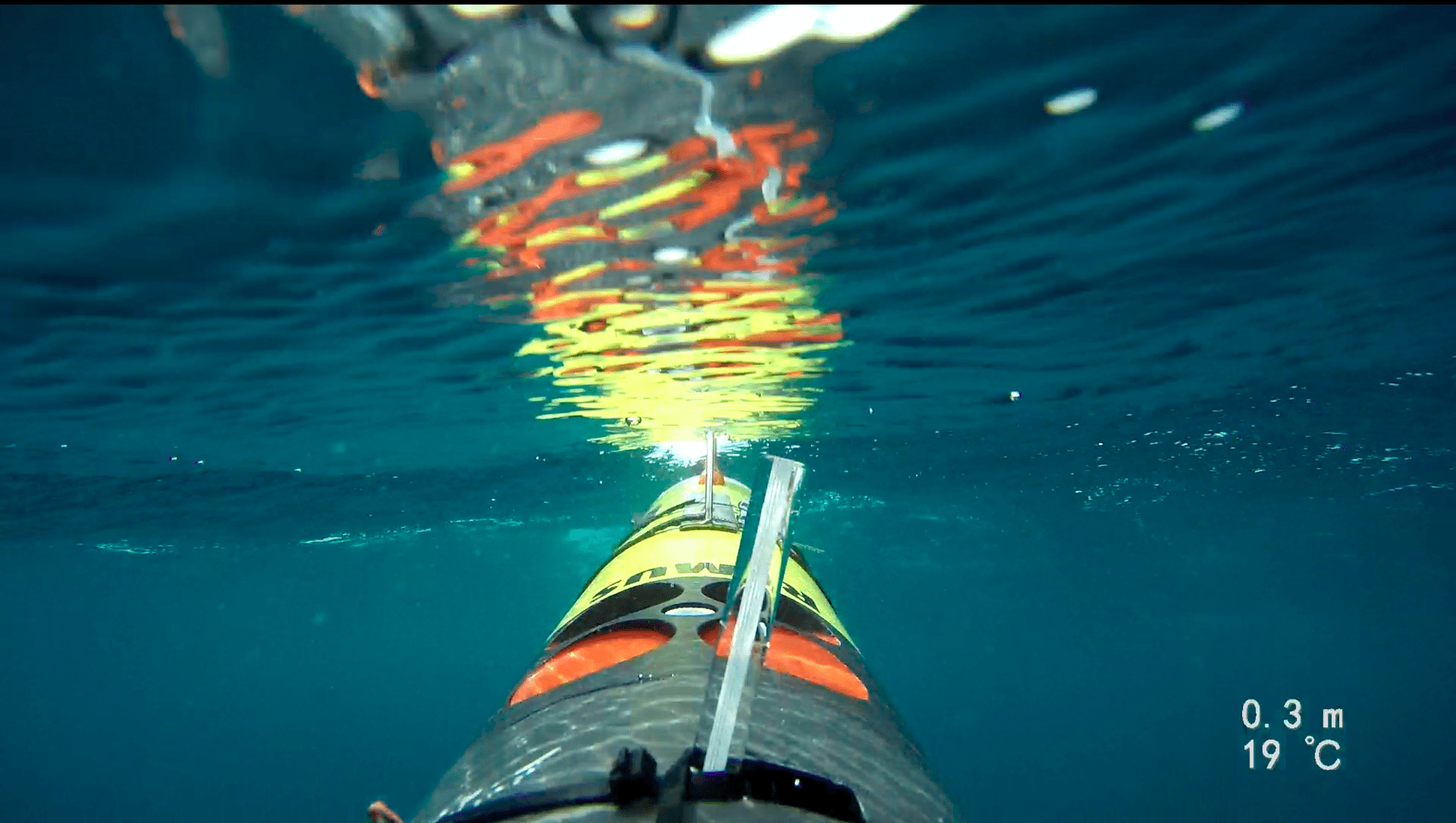
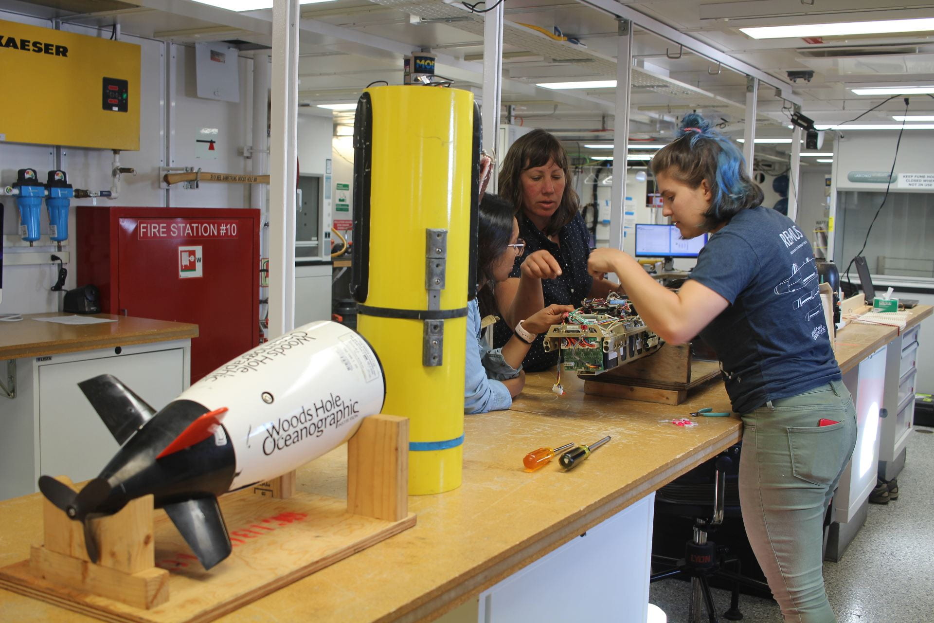
Polaris is our Long Range Autonomous Underwater Vehicle (LRAUV) developed by MBARI, different from the REMUS 100s not just in size and bright orange color, but in duration. The LRAUV was launched on Sunday of last week and with only a brief, couple of hours recovery on Friday to update code, the vehicle has been driving and gathering data on its own for the last ten days!

Polaris yo-yos through the water column measuring depth, temperature, salinity, dissolved oxygen, dissolved organic matter and light in the water. Every two hours it surfaces and uses satellite messages to send data back to shore, allowing the operators and scientists to monitor its progress and see a subset of the data it has collected. Using the same satellite messages, the operators can send commands and missions to the vehicle through a website on their phones. If anything goes wrong, Polaris will text them to let them know!

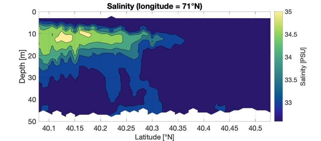
Polaris can be used to make lawnmower paths and cover a large area, but it is also capable of something more advanced—adaptive front tracking. When yo-yoing through a salinity intrusion, the salinity Polaris measures at 10, 20, 30, and 40 meters depths are very different from one another and are non-homogenous. When outside the intrusion, the salinity at these four depths are much more similar to one another, and are homogenous. Polaris uses this to determine if it is currently profiling through a salinity intrusion or not. When Polaris moves from a homogeneous salinity area, to a non-homogenous salinity area, it identifies the edge of the front. It continues to drive a certain distance and then turns around, heading back at an angle from its original direction until it hits the edge of the front again. This way it can move East or West, mapping the edge of the salinity intrusion!

 

To estimate ocean flows, oceanographers study horizontal density variations throughout the oceans. However, bringing water back to the surface and putting it on a scale to measure density is both costly and prone to errors. Thus, in 1969 Neil Brown (WHOI) invented an instrument that simultaneously measures Conductivity (to calculate salinity), Temperature, and Depth, called “CTD.” With these three variables on hand, one can calculate the density of ocean water. Over time more and more instruments and bottles for collecting water samples got attached to the CTD, and today research vessels carry a ~500kg heavy carousel full of instrumentation that is simply called the CTD.

The CTD is used to get a rough overview of the ocean column setup in a particular area. The carousel gets lowered over the side of the research vessel and the winch operator brings it down until about 5m above the ocean floor. Meanwhile, the computers on the science deck broadcast the measured profile live which allows the science party to decide where to take water samples on the way up.

Lets talk about Warm Core Rings , the very important R in SIRATES. Rings,  also referred to as eddies, are typically formed off a Gulf Stream meander. When the Gulf Stream detaches from the coast it begins to wiggle, when a large wiggle occurs it can pinch of and form a ring as pictured in the animation below. The rings that pinch off to the north are called Warm Core Rings due to the core of warm water from the Sargasso Sea. There are also rings that pinch off to the south with a cold slope water core called Cold Core Rings.

Once detached from the Gulf Stream, these rings move westward through the slope where they can hit the continental shelf. This is where rings become important for this project, transporting the  the warm salty water that form the salinity intrusions northward onto the shelf.

In our current study area an interesting phenomena is happening. Not only is there a warm anticyclonic (clockwise) ring against the shelf, there is an adjacent cyclonic (counter clockwise) ring to the southwest. This ring pair feature is called a mushroom, and is fairly uncommon this close to the shelf. It is thought that these rings might be working together to help strengthening the intrusions’ northward flow over the shelf.

 

 

 

Did anyone guess correctly?

This fighting squid tells more of a story then you might think, featuring every part of the our project’s name SIRATES ( Salinity Intrusions, Rings, AUVs, Turbulence, and Squid). The background contour is real data from one of the Darter missions (one of the REMUSs) showing a  salinity intrusion in light green in the upper right hand corner.  The fighting squid is riding an AUV (a mix between a REMUS and LRAUV) and holding a VMP (which measures turbulence) .  And of course we had to give the squid an eye patch.

What is the VMP?
The vertical microstructure profiler (VMP-250 by Rockland Scientific) is a loosely-tethered instrument which allows us to measure the small scales where energy dissipation and mixing occur. The profiler is equipped with two velocity-shear probes, so that turbulent kinetic energy (TKE) dissipation can be quantified even in well mixed areas. The shear probes are 8.5 mm long and 4.7 mm wide, and they directly measure small fluctuations in velocity-shear at a sampling rate of over 500 Hz. These probes can be thought of like record needles encased in silicone which measure tiny deflections due to the forces caused by fluctuations in velocity. The VMP also measures pressure (for depth), fluorescence (for chlorophyll-a), turbidity (for clarity), and conductivity (for salinity) with high precision and resolution.

How is the VMP deployed?
While the ship travels at 3-4 knots, the VMP is towed behind the vessel and “released” so that it free-falls vertically under its own negative buoyancy at a constant smooth velocity. This velocity is pre-determined by adjusting the weight of the profiler so that it falls at a velocity that optimizes the sampling resolution (in this case ~0.7 m/s). While the VMP is falling, the tether to the vessel must be slack, so that the motion of the ship is not felt by the instrument. When the VMP reaches the target depth (~50 meters for this experiment) it is retrieved using a deep sea electric fishing reel (Lundgren-Pitman S-1200) which pulls it back to the surface near the stern of the vessel, where it can be released again to take another profile at the new location. In this way we get a series of high resolution profiles in both space and time. This method of profiling s called “tow-yoing,” a combination of towing and yo-yoing.

What can we learn with the VMP?
Using the VMP, we will make high resolution measurements of temperature and velocity shear through the intrusions. These measurements enable us to determine the rate at which the intrusions are mixed and diffused by turbulence, which in turn plays a role in their onshore evolution and impact on shelf water mass properties. We will be looking out for wind events, internal tides, and solitary waves, all of which can generate shear and turbulence within the water column and potentially enhance the diffusion of the intrusions. We will also assess the competing role of thermohaline mixing via processes such as double diffusion and salt fingering in salinity intrusions.

Any guesses? Can you spot the salinity intrusion?

With one week down in the cruise and one to go we have some questions answered and many more generated. So far we have taken 32 CTD and  230 VMP casts and have covered 173.37 km with Polaris and   178.29 km with our two REMUS vehicles.  These measurements have helped to map two different salinity intrusions in our study region.

Below you can see a plot of the  temperature versus salinity measurements from all 32 of our CTD casts until now. Temperature-Salinity scatter plots help oceanographers identify the different water masses present in our profiles. Intrusion water looks very different than the surrounding shelf waters.  The intrusions are warm and salty, i.e., they appear in the upper right corner of the plot, whereas the shelf waters are cool and fresh and appear in the bottom left of the plot. The Z shaped profile is particularly unique to intrusion profiles. The relatively fresh but warm surface waters are in the upper limb of the ‘Z’, while the colder and saltier bottom waters follow along the lower limb of the ‘Z’.

 

In the Week to Come . . .  

• Front tracking with AUVs. This morning Polaris was launched once again after a short recovery to recharge and is now off on a new mission – this time using its front tracking algorithm. This will hopefully outline the intrusion and give us an idea of its extent.
• More CTDs and VMPs! The intrusion have been much patchier than expected and as much data as possible will be needed in order to get a complete 3D picture. The VMP’s turbulence measurements will also help us understand how long these features will last.
• Squid squid squid! Though our first attempts of squid jigging were unsuccessful,  we know they are out there and we will try again.

Today we sample a 40x40km area east of our home base along the 71°W longitude line. With CTD casts we want to get a first overview about the extent of a 2^nd intrusion area. While steaming to our next station, let’s take the time to feature our underwater robots of the REMUS family. We have 3 Remus-100’s with us on board the Armstrong, Darter, Edgar, and Sellers. These vehicles have a depth rating of 100 meters.

How do the REMUS missions work?

The vehicles communicate differently when at the surface and while underwater. At the surface, they’re use Wifi, make satellite phone calls, and get GPS coordinates from satellite. However, none of these systems work underwater and signals between the ship and the REMUS get transferred acoustically.

The vehicles are equipped with a variety of instruments to measure temperature, salinity, nitrate, dissolved organic matter, water velocity, and many variables more. In addition, we can make videos with a GoPro. Depending on the mission, the instrumentation can be adapted.

How does the AUV-Team’s day look like:

After a daily discussion with the science team, our AUV-Team (Amy, Noa, and Maaya) choose the best suited Remus for the day’s mission data goals and prepare the vehicle for deployment. A so-called Towfish, the 25kHz transducer used to acoustically communicate with the vehicles, is secured to the boat railing and lowered into the water prior to deployment. Once the vehicle is in the water and communications between us and the vehicle are established, we send the vehicle on its mission and stay within acoustic range until it’s time for recovery.

For more information on the AUV’s and the SciBotics team head to their website linked here.

Today had its ups and downs… 98 ups and downs to be precise: The VMP samples the water column like a yo-yo: Up and down… When releasing it, it falls down with a constant velocity and measures salinity, turbulent mixing, and many other variables. Then, we recover it with a motorized deep-sea fishing reel. One cast takes about 3min which allows great spatial resolution. Check out our salinity transact below.